Chimera States
Mircheski Petar
April 28, 2025
How Chimera States Adapt to Frequency Heterogeneity: A Self-Organizing Dance of Oscillators
Chimera states are one of the most intriguing phenomena in the world of nonlinear dynamics. They are composed of identical oscilaltors connected in a ring. Under certain conditions, they mysteriously split into two groups: one synchronized and coherent, the other disordered and chaotic. This coexistence of coherence and incoherence, is what defines a chimera state.
Originally reported by Kuramoto and Battogtokh in 2002 and named by Abrams and Strogatz in 2004, chimera states have fascinated scientists across disciplines. They've been observed in chemical reactions, mechanical systems, lasers, and more. Over the years, researchers have dug into how different types of connections, oscillator behaviors, and dimensional setups influence these states.
But what happens when the oscillators aren't quite identical? What if each one has a slightly different natural rhythm?
The Ring of Oscillators
We begin with a standard setup: a ring of phase oscillators, where each oscillator's behavior is described by a simple mathematical model.
These oscillators are connected nonlocally, each one of them feels the influence of its neighbors, but not just the immediate ones. The coupling strength is determined by the function , and the phase lag is given by . In our case we define a ring of 256 oscillators, connected through a cosine distance kernel,
and fix the system parameters to and .
from typing import Callable

import numba
import numpy as np


def cosine_kernel(A: float, N: int) -> np.ndarray:
    """
    Calculate the distance kernel delta_y for a system of oscillators.
    This function generates a coupling kernel based on a cosine function,
    which is then normalized.

    :param A: A scaling parameter that affects the coupling strength between oscillators.
    :param N: The number of spatial grid points, which corresponds to the number of oscillators.
    :returns: A 1D numpy array of length N containing the computed coupling kernel values, scaled to ensure normalization.
    """
    x = np.linspace(-np.pi, np.pi, N, endpoint=False)
    delta_y = (1 + A * np.cos(x)) / (2 * np.pi)
    kernel = delta_y * ((2 * np.pi) / N)
    return kernel


def cosine_kernel_fft(A: float, N: int) -> np.ndarray:
    """
    Calculate the FFT of the shifted cosine kernel for a system of oscillators.
    This function generates a coupling kernel based on a cosine function,
    shifts it for convolution purposes, and computes its FFT.

    :param A: A scaling parameter that affects the coupling strength between oscillators.
    :param N: The number of spatial grid points, which corresponds to the number of oscillators.
    :returns: A 1D numpy array of length N containing the FFT of the shifted coupling kernel.
    """
    kernel = cosine_kernel(A, N)
    # Shift the kernel for convolution theorem
    kernel_shifted = np.fft.ifftshift(kernel)
    kernel_fft = np.fft.fft(kernel_shifted)
    return kernel_fft


def kuramoto_kernel(
    omegas: np.ndarray | float,
    kernel_fft: np.ndarray,
    alpha: float,
) -> Callable[[np.ndarray], np.ndarray]:
    """
    Kuramoto model using FFT-based convolution.

    :param omega: Natural frequencies array (length N)
    :param alpha: Phase lag parameter
    :param kernel_fft: Precomputed FFT of the shifted coupling kernel
    """

    def f(theta: np.ndarray) -> np.ndarray:
        u = np.exp(1j * theta)  # e^{i\theta}

        # Z = G * e^{i\theta} via convolution theorem
        Z = np.fft.ifft(np.fft.fft(u) * kernel_fft)

        # Kuramoto coupling: Im[Z * e^{-i(\theta + \alpha)}]
        coupling = np.imag(Z * np.exp(-1j * (theta + alpha)))

        return omegas + coupling

    return f


np.random.seed(seed=1338)
N = 256
A = 0.995
alpha = (np.pi / 2) - 0.18
kernel_fft = cosine_kernel_fft(A, N)
dt = 0.1
In a perfectly uniform setup, the position of the chimera state on the ring is completely determined by the system's initial conditions. That's because the system is spatially homogeneous meaning, no location is special.
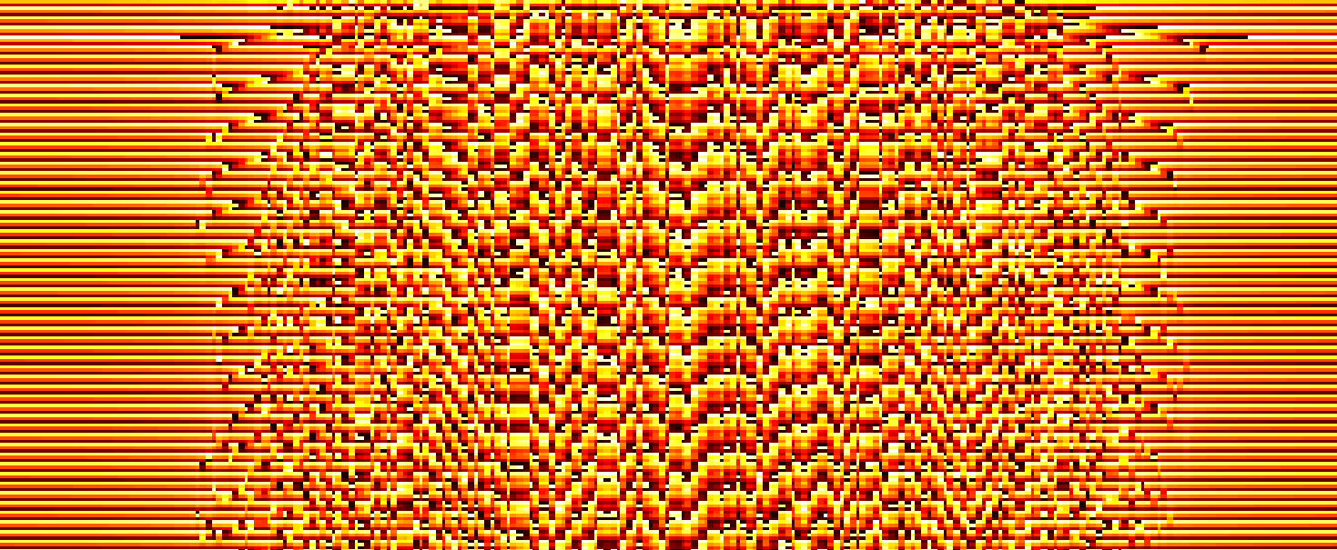
Chimera States Without Heterogeneity
We begin with this uniform system and observe the classic chimera behavior: a stable pattern with a coherent region and an incoherent region coexisting side by side. These patterns arise spontaneously and can be visualized in terms of phase snapshots, local coherence, and even instantaneous frequencies across the ring.
evolve_time = 500.0
t_evolve_eval = np.arange(0, evolve_time+dt, dt)
t_evolve_span =  (0, evolve_time+dt)

omegas = np.zeros(N)
initial_conditions = (
    6.0
    * np.exp(-0.76 * (np.linspace(-np.pi, np.pi, N, endpoint=False)) ** 2)
    * (np.random.random(N) - 0.5)
)

kuramoto = kuramoto_kernel(omegas, kernel_fft, alpha=alpha)
sol = solve_ivp(
    lambda t, y: kuramoto(y),
    t_evolve_span,
    initial_conditions,
    t_eval=t_evolve_eval,
    method="RK45",
    rtol=1e-7,
    atol=1e-10,
)
init_state = sol.y.T

fig, ax = plt.subplots(2, sharex=True)
heatmap = ax[0].imshow(
    init_state % (2 * np.pi), aspect="auto", interpolation="none", cmap="hot"
)

ax[0].set_ylabel(r"$t$")
ax[0].set_xlabel(r"$i$")
ax[0].set_title(r"$a)$", loc="left")


# Scatter plot
ax[1].scatter(np.arange(N), init_state[5000] % (2 * np.pi))
ax[1].set_xlabel(r"$i$")
ax[1].set_yticks([0, np.pi, 2 * np.pi])
ax[1].set_yticklabels([r"$0$", r"$\pi$", r"$2\pi$"])
ax[1].set_title(r"$b)$", loc="left")


cax = plt.axes((0.85, 0.1, 0.075, 0.8))
cbar = fig.colorbar(heatmap, cax=cax)
cbar.set_label(r"$\phi$")
cbar.set_ticks([0, np.pi / 2, np.pi, 3 * np.pi / 2, 2 * np.pi])
cbar.set_ticklabels(
    [r"$0$", r"$\frac{\pi}{2}$", r"$\pi$", r"$\frac{3\pi}{2}$", r"$2\pi$"]
)

plt.subplots_adjust(bottom=0.1, right=0.8, top=0.9)

plt.show()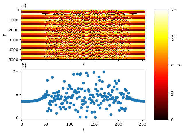
But what happens when we gently nudge the system out of uniformity?
Introducing Frequency Heterogeneity
To probe the system's adaptability, we introduce a small frequency heterogeneity—a subtle difference in the natural frequencies of the oscillators. This can be thought of as introducing a "preference" in certain parts of the ring. The mathematical form of this perturbation is:
Here, is a small number (think of it as a tiny tweak), and is a function that defines how the frequency varies in space. The parameter determines where this heterogeneity is placed on the ring.
We explore two types of heterogeneity:
1. Point heterogeneity
A spike at a single location.
new_omegas = np.zeros(N)
new_omegas[0] += 0.2

kuramoto = kuramoto_kernel(new_omegas, kernel_fft, alpha=alpha)

t_evolve_eval = np.arange(0, evolve_time * 6 + dt, dt)
t_evolve_span = (0, evolve_time * 6 + dt)

perturbed_sol = solve_ivp(
    lambda t, y: kuramoto(y),
    t_evolve_span,
    init_state[-1],
    t_eval=t_evolve_eval,
    method="RK45",
    rtol=1e-7,
    atol=1e-10,
)
perturbed_state = perturbed_sol.y.T

fig, ax = plt.subplots(2, sharex=True)
heatmap = ax[0].imshow(
    perturbed_state % (2 * np.pi), aspect="auto", interpolation="none", cmap="hot"
)

ax[0].set_ylabel(r"$t$")
ax[0].set_xlabel(r"$i$")
ax[0].set_title(r"$a)$", loc="left")


# Scatter plot
ax[1].scatter(np.arange(N), perturbed_state[-1] % (2 * np.pi))
ax[1].set_xlabel(r"$i$")
ax[1].set_yticks([0, np.pi, 2 * np.pi])
ax[1].set_yticklabels([r"$0$", r"$\pi$", r"$2\pi$"])
ax[1].set_title(r"$b)$", loc="left")


cax = plt.axes((0.85, 0.1, 0.075, 0.8))
cbar = fig.colorbar(heatmap, cax=cax)
cbar.set_label(r"$\phi$")
cbar.set_ticks([0, np.pi / 2, np.pi, 3 * np.pi / 2, 2 * np.pi])
cbar.set_ticklabels(
    [r"$0$", r"$\frac{\pi}{2}$", r"$\pi$", r"$\frac{3\pi}{2}$", r"$2\pi$"]
)

plt.subplots_adjust(bottom=0.1, right=0.8, top=0.9)

plt.show()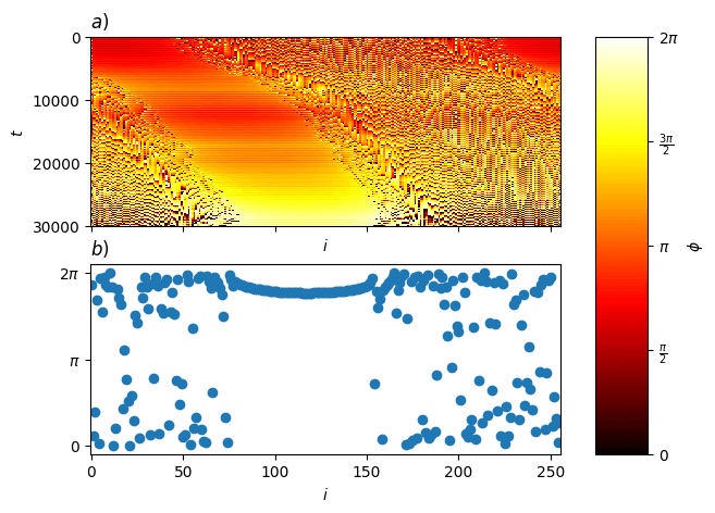
2. Cosine heterogeneity
x = np.linspace(-np.pi, np.pi, N, endpoint=False)
new_omegas = 0.01 * np.cos(x + np.pi)
kuramoto = kuramoto_kernel(new_omegas, kernel_fft, alpha=alpha)

t_evolve_eval = np.arange(0, evolve_time * 3 + dt, dt)
t_evolve_span = (0, evolve_time * 3 + dt)

perturbed_sol = solve_ivp(
    lambda t, y: kuramoto(y),
    t_evolve_span,
    init_state[-1],
    t_eval=t_evolve_eval,
    method="RK45",
    rtol=1e-7,
    atol=1e-10,
)
perturbed_state = perturbed_sol.y.T

fig, ax = plt.subplots(2, sharex=True)
heatmap = ax[0].imshow(
    perturbed_state % (2 * np.pi), aspect="auto", interpolation="none", cmap="hot"
)

ax[0].set_ylabel(r"$t$")
ax[0].set_xlabel(r"$i$")
ax[0].set_title(r"$a)$", loc="left")


# Scatter plot
ax[1].scatter(np.arange(N), perturbed_state[-1] % (2 * np.pi))
ax[1].set_xlabel(r"$i$")
ax[1].set_yticks([0, np.pi, 2 * np.pi])
ax[1].set_yticklabels([r"$0$", r"$\pi$", r"$2\pi$"])
ax[1].set_title(r"$b)$", loc="left")


cax = plt.axes((0.85, 0.1, 0.075, 0.8))
cbar = fig.colorbar(heatmap, cax=cax)
cbar.set_label(r"$\phi$")
cbar.set_ticks([0, np.pi / 2, np.pi, 3 * np.pi / 2, 2 * np.pi])
cbar.set_ticklabels(
    [r"$0$", r"$\frac{\pi}{2}$", r"$\pi$", r"$\frac{3\pi}{2}$", r"$2\pi$"]
)

plt.subplots_adjust(bottom=0.1, right=0.8, top=0.9)

plt.show()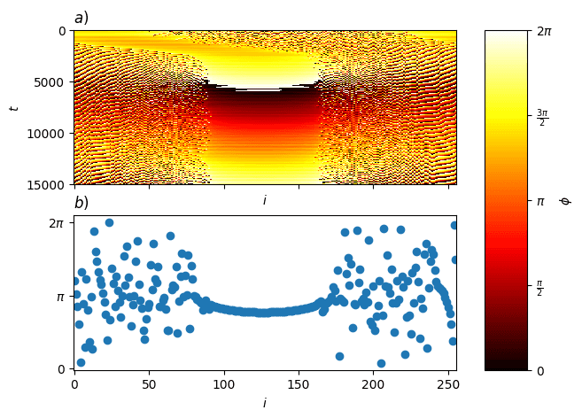
The Self-Adaptive Behavior of Chimera States
When we introduce point heterogeneity (like a single oscillator ticking faster), the chimera state responds in a surprising but consistent way. The incoherent region starts drifting—migrating toward the faster oscillator. Meanwhile, the coherent region drifts in the opposite direction, settling in the slower area.
This movement continues until the system reaches a new equilibrium, where the incoherent region hugs the heterogeneity, and the coherent region finds its new home far away from it.
When we switch to the smoother cosine heterogeneity, the same behavior emerges only this time, more gracefully. The incoherent region moves toward the high-frequency side of the cosine wave, while the coherent region moves toward the low-frequency trough. Again, a new steady state is reached, but now perfectly aligned with the shape of the heterogeneity.
Coherence Loves Low Frequencies
The takeaway from all of this? Regardless of how the heterogeneity is shaped—spiky or smooth—the chimera state adapts in the same fundamental way:
- Incoherent regions gravitate toward high natural frequencies.
- Coherent regions drift toward low natural frequencies.
This self-adaptive behavior is both robust and elegant. It shows that even in complex dynamical systems, a simple principle can emerge: the system self-organizes in a way that aligns its internal structure with the external heterogeneity.
We call this phenomenon spatial phase locking to frequency heterogeneity.
Why Does This Matter?
Understanding how chimera states adapt to heterogeneity has implications in various fields. Knowing how these patterns respond to imperfections or design tweaks could help us control, harness, or stabilize such systems in the real world.